In machine learning, the perceptron is an algorithm for the controlled learning of binary classifiers. It is also often called the perceptron. A binary classifier is a function that can decide whether an input represented by a vector of numbers belongs to a particular class. This is a type of linear classifier, that is, a classification algorithm that makes its predictions based on a linear predictor function that combines a set of weights with a feature vector.
In recent years, artificial neural networks have attracted attention thanks to advances in deep learning. But what is an artificial neural network and what does it consist of?
Meet the perceptron
In this article, we briefly look at artificial neural networks in general, then look at one neuron, and finally (this is part of the coding), we take the most basic version of an artificial neuron, the perceptron, and classify its points on the plane.
Have you ever wondered why there are tasks that are so simple for any person, but incredibly difficult for computers? Artificial neural networks (abbreviated ANN) were inspired by the human central nervous system. Like their biological counterpart, ANNs are built on simple signal processing elements that are combined into a large grid.
Neural networks must learn
Unlike traditional algorithms, neural networks cannot be “programmed” or “configured” for their intended purpose. Like the human brain, they must learn to complete the task. Roughly speaking, there are three learning strategies.
The simplest method can be used if there is a test data set (large enough) with known results. Then the training goes like this: process one data set. Compare the result with the known result. Configure the network and retry. This is the learning strategy we will use here.
Unsupervised learning
Useful if there is no test data available and if it is possible to get any cost function from the desired behavior. The cost function tells the neural network how far it is from the target. Then the network can adjust its parameters on the fly, working with real data.
Enhanced learning
The carrot and stick method. It can be used if the neural network generates continuous action. Over time, the network learns to prefer the right actions and avoid the wrong ones.
Well, now we know a little about the nature of artificial neural networks, but what exactly are they made of? What will we see if we open the lid and look inside?
Neurons are the building blocks of neural networks. The main component of any artificial neural network is an artificial neuron. They are not only named after their biological counterparts, but also modeled on the behavior of neurons in our brain.
Biology vs. Technology
Just like a biological neuron has dendrites for receiving signals, a cell body for processing them and an axon for sending signals to other neurons, an artificial neuron has several input channels, a processing stage and one output that can branch out to many other artificial neurons.
Can we do something useful with one perceptron? There is a class of problems that one perceptron can solve. Consider the input vector as the coordinates of the point. For a vector with n-elements, this point will live in n-dimensional space. To simplify life (and the code below), let's assume that it is two-dimensional. Like a piece of paper.
Next, imagine that we draw several random points on this plane and divide them into two sets, drawing a straight line through the paper. This line divides the points into two sets, one above and the other below the line. The two sets are then called linearly separable.
One perceptron, no matter how simple it may seem, is able to find out where this line is, and when he finishes training, he can determine whether a given point is above or below this line.
History of invention
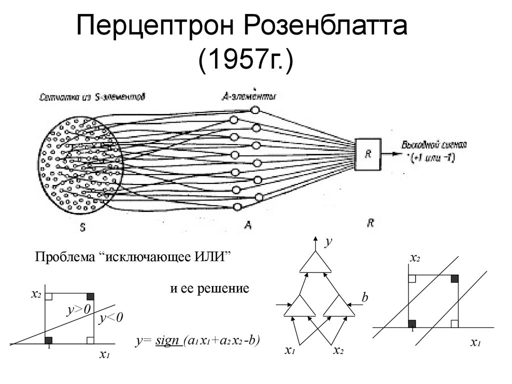
An algorithm for this method was invented in 1957 at the Cornell Aviation Laboratory by Frank Rosenblatt (a perceptron is often named after him), funded by the United States Naval Research Office. The perceptron was supposed to be a machine, not a program, and although its first implementation was in software for the IBM 704, it was subsequently implemented on custom hardware as a “brand 1 perceptron.” This machine was designed for image recognition: it had an array of 400 photocells randomly connected to neurons. The weights were encoded in potentiometers, and the weight update during training was performed by electric motors.
At a press conference organized by the US Navy in 1958, Rosenblatt made statements about the perceptron, which caused fierce debate among the young AI community; Based on Rosenblatt’s statements, the New York Times reported that the perceptron is "the germ of an electronic computer that the navy expects to be able to walk, talk, see, write, reproduce itself and be aware of its existence."
Further developments
Although the perceptron initially seemed promising, it was quickly proved that perceptrons could not be trained to recognize many classes of patterns. This led to stagnation in neural network perceptron research for many years before it was recognized that a neural network directly connected to two or more layers (also called a multilayer perceptron) had much greater processing power than single-layer perceptrons (also called a single perceptron layer). A single-layer perceptron is able to study only linearly separable structures. In 1969, the famous book by Marvin Minsky and Seymour Papert, Perceptrons, showed that these classes of networks cannot study the XOR function. However, this does not apply to nonlinear classification functions that can be used in a single-layer perceptron.
The use of such functions expands the capabilities of the perceptron, including the implementation of the XOR function. It is often believed (incorrectly) that they also assumed that a similar result would occur for a multilayer perceptron network. However, this is not so, since both Minsky and Papert already knew that multilayer perceptrons are capable of producing the XOR function. Three years later, Steven Grossberg published a series of papers representing networks capable of modeling differential functions, contrast enhancement functions, and XOR functions.
The works were published in 1972 and 1973. Nevertheless, the often skipped text of Minsky / Papert caused a significant decrease in interest and funding for research using the perceptron of neural networks. Another ten years passed until neural network research was revived in the 1980s.
Features
The perceptron core algorithm was introduced in 1964 by Aizerman et al. Limit boundary guarantees were given for the perceptron algorithm in the general inseparable case, first by Freind and Shapir (1998), and more recently by Mori and Rostamizade (2013), which extend the previous results and give new boundaries L1 .
Perceptron is a simplified model of a biological neuron. Although the complexity of biological neural models is often required to fully understand neural behavior, studies show that a perceptron-like linear model can cause some behavior observed in real neurons.
The perceptron is a linear classifier, so it will never get into a state with all input vectors classified correctly if the training set D is not linearly separable, i.e. if positive examples cannot be separated from negative examples by a hyperplane. In this case, no “rough” solution will pass gradually according to the standard learning algorithm, instead, training will fail completely. Therefore, if the linear separability of the training set is a priori unknown, use one of the training options below.
Pocket algorithm
The pocket algorithm with a ratchet mechanism solves the problem of sustainability of training with the perceptron, keeping the best of the solutions so far found “in the pocket”. The pocket algorithm then returns the solution in the pocket, not the last solution. It can also be used for inseparable data sets, where the goal is to search for a perceptron with a small number of erroneous classifications. Nevertheless, these solutions look stochastic and, therefore, the pocket algorithm does not gradually approach them in the learning process, and they are unwarrantedly detected during a certain number of learning stages.
Maxover Algorithm
Maxover’s algorithm is “stable” in the sense that it will converge regardless of knowledge of the linear separability of the data set. In the case of linear separation, this will solve the problem of learning, if desired, even with optimal stability (maximum margin between classes). For inseparable datasets, a solution with a small number of erroneous classifications will be returned. In all cases, the algorithm gradually approaches the solution in the learning process, without remembering previous states and without random jumps. Convergence lies in global optimality for shared datasets and in local optimality for inseparable datasets.
Voted perceptron
The Voted Perceptron algorithm is an option using multiple weighted perceptrons. The algorithm launches a new perceptron every time an example is erroneously classified, initializing the weight vector with the final weights of the last perceptron. Each perceptron will also be assigned a different weight, corresponding to how many examples they correctly classify before mistakenly classifying one, and at the end there will be a weighted vote on the entire perceptron.
Application
In separable problems, perceptron training can also be aimed at finding the largest separation boundary between classes. The so-called perceptron of optimal stability can be determined using iterative learning and optimization schemes, such as the Min-Over algorithm or AdaTron. AdaTron uses the fact that the corresponding quadratic optimization problem is convex. The perceptron of optimal stability together with the kernel trick are the conceptual basis of the support vector machine.
Alternative
Another way to solve non-linear problems without using multiple layers is to use higher-order networks (sigma-pi block). In a network of this type, each element of the input vector is expanded by each pairwise combination of multiplied inputs (second order). It can be expanded to an n-order network. Perceptron is a very flexible thing.
However, it should be remembered that the best classifier is not necessarily the one that accurately classifies all training data. Indeed, if we had a preliminary restriction on the fact that the data comes from equidistant Gaussian distributions, the linear separation in the input space is optimal, and the nonlinear solution is redefined.
Other linear classification algorithms include Winnow, a reference vector, and logistic regression. Perceptron is a universal set of algorithms.
Primary Application - Supervised Learning
Supervised learning is a machine learning task consisting in learning a function that maps input to output based on examples of input / output pairs. They derive a function from the labeled training data, consisting of a set of examples. In supervised learning, each example is a pair consisting of an input object (usually a vector) and a desired output value (also called a telltale).
The supervised learning algorithm analyzes the learning data and provides the intended function that can be used to display new examples. The optimal scenario will allow the algorithm to correctly determine class labels for invisible instances. This requires the learning algorithm to generalize learning data to invisible situations in a “reasonable” way.
A parallel task in human and animal psychology is often called conceptual learning.