👨🏻‍⚖️ 👆🏽 💌 Matrices: Gauss method. Gaussian Matrix Calculation: Examples ‼️ 🛸 🔲

Linear algebra, which is taught in universities in different specialties, combines many difficult topics. Some of them are related to matrices, as well as to solving systems of linear equations by the Gauss and Gauss - Jordan methods. Not all students manage to understand these topics, algorithms for solving various problems. Let's look at the matrices and methods of Gauss and Gauss - Jordan together.

Basic concepts

A matrix in linear algebra is a rectangular array of elements (table). Below are sets of elements enclosed in parentheses. This is the matrix. From the above example, it is clear that the elements in rectangular arrays are not only numbers. A matrix may consist of mathematical functions, algebraic symbols.

In order to deal with some concepts, we compose a matrix A from the elements a _ij . Indexes are not just letters: i is the number of the row in the table, and j is the number of the column in the intersection area of which is located the element a _ij . So, we see that we have obtained a matrix of such elements as a ₁₁ , a ₂₁ , a ₁₂ , a ₂₂ , etc. The letter n denotes the number of columns, and the letter m denotes the number of rows. The symbol m × n denotes the dimension of the matrix. This is the concept that defines the number of rows and columns in a rectangular array of elements.

Optionally, the matrix must have multiple columns and rows. At a dimension of 1 × n, the array of elements is single-line, and at a dimension of m × 1, it is single-column. If the number of rows and the number of columns is equal, the matrix is called square. Each square matrix has a determinant (det A). This term refers to a number that is assigned to the matrix A.

A few more important concepts that you need to remember to successfully solve matrices are the main and secondary diagonals. By the main diagonal of a matrix is meant that diagonal that goes down to the right corner of the table from the left corner from above. The side diagonal goes to the right corner up from the left corner from below.

Stepped view of the matrix

Take a look at the picture below. On it you will see a matrix and a circuit. We will first deal with the matrix. In linear algebra, a matrix of this kind is called stepwise. One property is inherent in it: if a _ij is the first nonzero element in the ith row, then all other elements from the matrix that are lower and to the left of a _ij are zero (i.e., all those elements that can be given the letter notation a _kl , where k> i, and l <j).

Now consider the circuit. It reflects the stepped shape of the matrix. The scheme presents 3 types of cells. Each view denotes certain elements:

empty cells - zero elements of the matrix;
shaded cells are arbitrary elements that can be either zero or nonzero;
black squares are nonzero elements, which are called corner elements, “steps” (in the matrix presented nearby, such elements are the numbers –1, 5, 3, 8).

When solving matrices, sometimes such a result is obtained when the "length" of the step is greater than 1. This is allowed. Only the "height" of the steps is important. In a stepped matrix, this parameter should always be equal to unity.

Reduction of a matrix to a step form

Any rectangular matrix can be converted to a stepped view. This is done thanks to elementary transformations. They include:

permutation of lines in places;
adding to one line another line, if necessary multiplied by any number (you can also perform the subtraction operation).

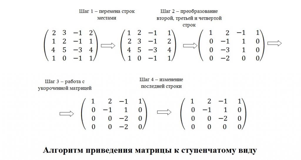
Consider elementary transformations in solving a specific problem. The figure below shows the matrix A, which must be reduced to a stepwise form.

The task of reducing the matrix to a stepwise form

In order to solve the problem, we will follow the algorithm:

It is convenient to perform transformations on such a matrix in which the first element in the upper corner on the left side (that is, the “leading” element) is 1 or –1. In our case, the first element in the top line is 2, so we swap the first and second lines in places.
We perform the subtraction operations, touching rows No. 2, 3, and 4. We should get zeros in the first column under the “leading” element. To achieve this result: from the elements of line number 2, we subtract the elements of line number 1 multiplied by 2; from the elements of line number 3, we sequentially subtract the elements of line number 1 multiplied by 4; from the elements of line number 4, we sequentially subtract the elements of line number 1.
Next, we will work with a shortened matrix (without column No. 1 and without row No. 1). The new “lead” element at the intersection of the second column and second row is –1. You do not need to rearrange the rows, so we rewrite the first column and the first and second rows without changes. We perform subtraction operations in order to get zeros in the second column under the “leading” element: from the elements of the third line, we subtract the elements of the second line multiplied by 3; from the elements of the fourth line we sequentially subtract the elements of the second line multiplied by 2.
It remains to change the last line. From its elements we subtract successively the elements of the third row. So we got a step matrix.

The reduction of matrices to step form is used in solving systems of linear equations (SLE) by the Gauss method. Before considering this method, let's look at terms related to SLE.

Matrices and systems of linear equations

Matrices are used in various sciences. Using tables of numbers it is possible, for example, to solve linear equations combined in a system using the Gauss method. To get started, let's get acquainted with several terms and their definitions, and also see how a matrix is composed of a system that combines several linear equations.

SLU - several combined algebraic equations in which the unknowns are present in the first degree and there are no terms representing the product of the unknowns.

The solution of the SLU is the found values of the unknowns, the substitution of which equations in the system become identities.

Joint SLU is a system of equations that has at least one solution.

Incompatible SLU - a system of equations that has no solutions.

How is a matrix compiled on the basis of a system combining linear equations? There are such concepts as the basic and advanced matrix system. In order to get the main matrix of the system, it is necessary to put out all the coefficients for unknowns in the table. The expanded matrix is obtained by joining the column of free terms to the main matrix (it includes known elements to which each equation is equated). You can understand the whole process by examining the picture below.

The first thing we see in the picture is a system that includes linear equations. Its elements: a _ij are numerical coefficients, x _j are unknown quantities, b _i are free terms (where i = 1, 2, ..., m, and j = 1, 2, ..., n). The second element in the picture is the main matrix of coefficients. From each equation, the coefficients are written in a row. As a result, we get as many rows in the matrix as there are equations in the system. The number of columns is equal to the largest number of coefficients in any equation. The third element in the picture is an expanded matrix with a column of free terms.

Matrices and a system of linear equations

General Information on the Gauss Method

In linear algebra, the Gauss method is the classical method for solving SLUs. It bears the name of Karl Friedrich Gauss, who lived in the XVIII-XIX centuries. This is one of the greatest mathematicians of all time. The essence of the Gauss method is to perform elementary transformations on a system of linear algebraic equations. With the help of transformations, SLE is reduced to an equivalent system of a triangular (step) form, from which all variables can be found.

It is worth noting that Karl Friedrich Gauss is not the discoverer of the classical way of solving a system of linear equations. The method was invented much earlier. His first description is found in the encyclopedia of knowledge of ancient Chinese mathematicians, called "Mathematics in 9 books."

Gauss solution example

Consider a concrete example of the solution of systems by the Gauss method. We will work with the SLU presented in the picture.

Solution Algorithm:

By direct course of the Gauss method, we bring the system to a stepwise form, but for a start we will make an expanded matrix of numerical coefficients and free terms.
To solve the matrix by the Gauss method (i.e., bring it to a stepwise form), we subtract the elements of the first line from the elements of the second and third lines. We will get zeros in the first column under the “leading” element. Next, change the second and third lines in order for convenience. To the elements of the last row we add sequentially the elements of the second line multiplied by 3.
As a result of calculating the matrix by the Gauss method, we obtained a stepwise array of elements. Based on it, we will compose a new system of linear equations. By reversing the Gauss method, we find the values of the unknown members. The last linear equation shows that x ₃ is 1. Substitute this value in the second line of the system. This gives the equation x ₂ - 4 = –4. It follows that x ₂ is 0. Substitute x ₂ and x ₃ into the first equation of the system: x ₁ + 0 +3 = 2. The unknown term is –1.

Answer: using a matrix, the Gauss method, we found the values of the unknowns; x ₁ = –1, x ₂ = 0, x ₃ = 1.

Gauss-Jordan Method

In linear algebra there is also such a thing as the Gauss - Jordan method. It is considered a modification of the Gauss method and is used to find the inverse matrix, to calculate the unknown members of square systems of linear algebraic equations. The Gauss - Jordan method is convenient in that it allows you to solve SLS in one step (without using forward and reverse moves).

Let's start with the term inverse matrix. Suppose we have a matrix A. The matrix A ⁻¹ will be the inverse of it, and the condition A × A ⁻¹ = A ⁻¹ × A = E is necessarily satisfied, i.e., the product of these matrices is equal to the identity matrix (the identity matrix matrices, the elements of the main diagonal are units, and the remaining elements are equal to zero).

An important nuance: in linear algebra there is a theorem on the existence of an inverse matrix. A sufficient and necessary condition for the existence of the matrix A ^-1 is the non-degeneracy of A. When non-degenerate, det A (determinant) is not equal to zero.

The main steps on which the Gauss - Jordan method is based:

Take a look at the first row of a specific matrix. The Gauss-Jordan method can begin to be applied if the first value is not equal to zero. If the first place is 0, then swap the lines so that the first element has a non-zero value (it is desirable that the number be closer to one).
Divide all the elements of the first line by the first number. You get a line that starts with one.
Subtract the first line from the second line, multiplied by the first element of the second line, i.e. as a result, you get a line that starts from zero. Perform the same steps with the rest of the lines. In order to get units diagonally, divide each line by its first nonzero element.
As a result, you will get the upper triangular matrix by the Gauss - Jordan method. In it, the main diagonal is represented by units. The bottom corner is filled with zeros, and the top corner with a variety of values.
From the penultimate line, subtract the last line multiplied by the required coefficient. You should get a string with zeros and ones. For the remaining lines, repeat the same action. After all the transformations, we get the identity matrix.

An example of finding the inverse matrix by the Gauss - Jordan method

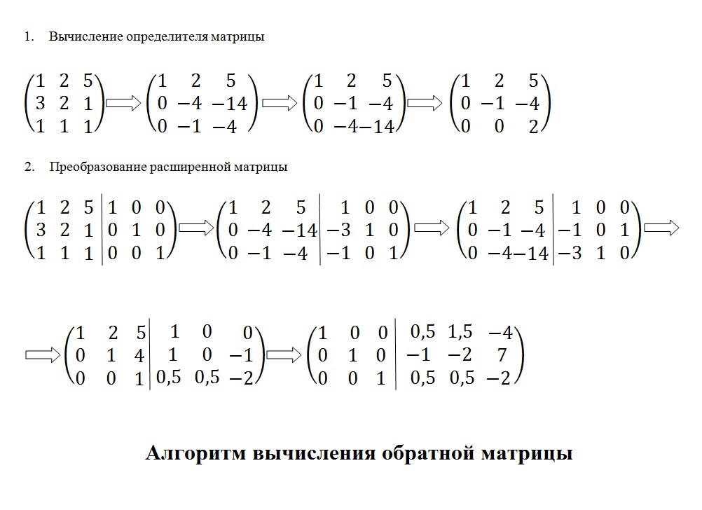
To calculate the inverse matrix, we need to write the extended matrix A | E and perform the necessary transformations. Consider a simple example. The figure below shows the matrix A.

The task of computing the inverse matrix

Decision:

First, find the determinant of the matrix by the Gauss method (det A). If this parameter is not equal to zero, then the matrix will be considered non-degenerate. This will allow us to conclude that A definitely has A ^-1 . To calculate the determinant, we transform the matrix to a step form by elementary transformations. We calculate the number K equal to the number of row permutations. We swapped lines only 1 time. We calculate the determinant. Its value will be equal to the product of the elements of the main diagonal multiplied by (–1) ^K. The result of the calculation: det A = 2.
We compose an expanded matrix by adding a unit matrix to the original matrix. The resulting array of elements will be used to find the inverse matrix by the Gauss - Jordan method.
The first element in the first line is one. This suits us, because we do not need to rearrange the lines and divide the given line by any number. We begin to work with the second and third lines. To make the first element in the second line turn to 0, subtract the first line multiplied by 3 from the second line. Subtract the first line from the third line (no multiplication required).
In the resulting matrix, the second element of the second line is –4, and the second element of the third line is –1. Swap the lines for convenience. Subtract the second line multiplied by 4. From the third line, divide the second line by –1, and the third line by 2. We get the upper triangular matrix.
From the second line, we subtract the last line, multiplied by 4, from the first line, the last line, multiplied by 5. Next, we subtract from the first line the second line, multiplied by 2. On the left side, we get the identity matrix. On the right is the inverse matrix.

An example of a solution to the SLS by the Gauss - Jordan method

The figure shows a system of linear equations. It is required to find the values of unknown variables using a matrix, the Gauss-Jordan method.

Decision:

We compose an expanded matrix. To do this, we put out the coefficients and free terms in the table.
We solve the matrix by the Gauss - Jordan method. Subtract row No. 1 from row No. 2. Subtract row number 1, previously multiplied by 2, from row No. 3.
We swap lines No. 2 and 3.
From line No. 3, subtract line No. 2 multiplied by 2. Divide the resulting third line by –1.
From line No. 2, subtract line No. 3.
From line No. 1, subtract line No. 2 times -1. On the side we got a column consisting of the numbers 0, 1 and –1. From this we conclude that x ₁ = 0, x ₂ = 1 and x ₃ = –1.

If desired, you can verify the correctness of the solution by substituting the calculated values in the equation:

0 - 1 = –1, the first identity from the system is true;
0 + 1 + (–1) = 0, the second identity from the system is true;
0 - 1 + (–1) = –2, the third identity from the system is true.

Conclusion: using the Gauss - Jordan method, we found the correct solution to a quadratic system combining linear algebraic equations.

Online calculators

The life of modern youth studying in universities and studying linear algebra has been greatly simplified. A few years ago, it was necessary to find solutions to systems by the Gauss and Gauss - Jordan methods independently. Some students successfully coped with the tasks, while others were confused in the decision, made mistakes, asked classmates for help. Today you can use online calculators when doing your homework. To solve systems of linear equations, search for inverse matrices, programs have been written that demonstrate not only the correct answers, but also show the progress of solving a particular problem.

There are many resources on the Internet with built-in online calculators. Matrices by the Gauss method, systems of equations are solved by these programs in a few seconds. Students only need to specify the necessary parameters (for example, the number of equations, the number of variables).

Matrices: Gauss method. Gaussian Matrix Calculation: Examples