In this article, the method is considered as a method of solving systems of linear equations (SLAE). The method is analytical, that is, it allows you to write a solution algorithm in a general form, and then substitute the values from specific examples there. Unlike the matrix method or Cramer's formulas, when solving a system of linear equations by the Gauss method, you can work with those that have infinitely many solutions. Or don't have it at all.
What does it mean to solve by the Gauss method?
First you need to write our system of equations in the form of a matrix. It looks as follows. The system is taken:
The coefficients are written in the form of a table, and on the right, in a separate column, are free terms. A column with free members is separated for convenience by a vertical bar. The matrix that includes this column is called extended.
Next, the main matrix with the coefficients must be reduced to the upper triangular form. This is the main point of solving the system by the Gauss method. Simply put, after certain manipulations, the matrix should look so that there are only zeros in its lower left part:
Then, if we write the new matrix again as a system of equations, we can see that the last line already contains the value of one of the roots, which is then substituted into the equation above, there is another root, and so on.
This is a description of the solution by the Gauss method in its most general terms. And what happens if the system suddenly has no solution? Or are there infinitely many? To answer these and many more questions, it is necessary to consider separately all the elements used in solving the Gauss method.
Matrices, their properties
There is no hidden meaning in the matrix. This is just a convenient way to record data for subsequent operations with them. Even schoolchildren do not need to be afraid of them.
The matrix is always rectangular, because it is more convenient. Even in the Gauss method, where it all comes down to constructing a matrix of a triangular form, a rectangle appears in the record, only with zeros in the place where there are no numbers. Zeros can be omitted, but they are implied.
The matrix has a size. Its "width" is the number of rows (m), "length" is the number of columns (n). Then the size of the matrix A (Latin letters are usually used for their designation) will be denoted as A m × n . If m = n, then this matrix is square, and m = n is its order. Accordingly, any element of the matrix A can be denoted by the number of its row and column: a xy ; x - row number, changes [1, m], y - column number, changes [1, n].
In the Gauss method, matrices are not the main point of the solution. In principle, all operations can be performed directly with the equations themselves, but the record will be much more cumbersome, and it will be much easier to get confused.
Determinant
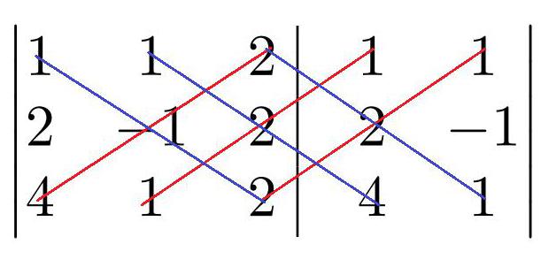
The matrix also has a determinant. This is a very important feature. It’s not worth figuring out its meaning now, you can just show how it is calculated, and then tell what properties of the matrix it determines. The easiest way to find the determinant is through the diagonals. The matrix draws imaginary diagonals; the elements located on each of them are multiplied, and then the resulting products are added up: diagonals with a slope to the right - with a plus sign, with a slope to the left - with a minus sign.
It is extremely important to note that the determinant can be calculated only on a square matrix. For a rectangular matrix, you can do the following: from the number of rows and the number of columns, select the smallest (let it be k), and then arbitrarily mark k columns and k rows in the matrix. Elements at the intersection of selected columns and rows will make up a new square matrix. If the determinant of such a matrix is a number other than zero, then it will be called the base minor of the initial rectangular matrix.
Before proceeding to the solution of the system of equations by the Gauss method, the determinant does not interfere. If it turns out to be zero, then we can immediately say that the number of solutions in the matrix is either infinite, or none at all. In such a sad case, you need to go further and find out about the rank of the matrix.
System classification
There is such a thing as the rank of a matrix. This is the maximum order of its determinant, nonzero (if we recall the basis minor, we can say that the rank of the matrix is the order of the basis minor).
By the way things are with the rank, SLAU can be divided into:
- Joint. In joint systems, the rank of the main matrix (consisting only of coefficients) coincides with the rank of the extended (with a column of free terms). Such systems have a solution, but not necessarily one, so additionally joint systems are divided into:
- - certain - having a single solution. In certain systems, the matrix rank and the number of unknowns (or the number of columns, which are one and the same) are equal;
- - indefinite - with an infinite number of solutions. The rank of matrices in such systems is less than the number of unknowns.
- Incompatible. For such systems, the ranks of the main and extended matrices do not coincide. Incompatible systems have no solution.
The Gauss method is good because it allows one to obtain in the course of a solution either an unambiguous proof of the incompatibility of the system (without calculating the determinants of large matrices), or a general solution for a system with an infinite number of solutions.
Elementary transformations
Before proceeding directly to the solution of the system, you can make it less cumbersome and more convenient for calculations. This is achieved through elementary transformations - such that their implementation does not change the final answer. It should be noted that some of the above elementary transformations are valid only for matrices, the source of which was precisely SLAE. Here is a list of these conversions:
- Permutation of lines. Obviously, if you change the order of the equations in the system record, then this will not affect the solution in any way. Therefore, in the matrix of this system it is also possible to interchange the rows, without forgetting, of course, about the column of free terms.
- Multiplication of all elements of the string by a certain factor. Very helpful! With it, you can reduce large numbers in the matrix or remove zeros. Many solutions, as usual, will not change, and it will become more convenient to perform further operations. The main thing is that the coefficient is not equal to zero.
- Delete rows with proportional coefficients. This partly follows from the previous paragraph. If two or more rows in the matrix have proportional coefficients, then when multiplying / dividing one of the rows by the proportionality coefficient, two (or, again, more) absolutely identical rows are obtained, and you can remove the extra ones, leaving only one.
- Deletion of a zero line. If during the transformations somewhere we get a row in which all elements, including the free term, are zero, then such a row can be called zero and thrown out of the matrix.
- Adding to the elements of one row the elements of another (in the corresponding columns) multiplied by a certain coefficient. The most unobvious and most important transformation of all. It should dwell in more detail.
Adding a line multiplied by a factor
For ease of understanding, it is worth taking this process step by step. Two rows from the matrix are taken:
a 11 a 12 ... a 1n | b1
a 21 a 22 ... a 2n | b 2
Suppose you want to add the first one multiplied by the coefficient "-2" to the second.
a '21 = a 21 + -2 × a 11
a '22 = a 22 + -2 × a 12
...
a ' 2n = a 2n + -2 × a 1n
Then, in the matrix, the second row is replaced with a new one, and the first remains unchanged.
a 11 a 12 ... a 1n | b1
a '21 a' 22 ... a ' 2n | b 2
It should be noted that the multiplication factor can be chosen so that as a result of adding two lines, one of the elements of the new line is equal to zero. Therefore, it is possible to obtain an equation in a system where one unknown is less. And if you get two such equations, then the operation can be done again and get an equation that will already contain two less unknowns. And if each time you turn one coefficient into zero for all rows, which are lower than the original, you can, as steps go down to the very bottom of the matrix and get an equation with one unknown. This is called solving the system by the Gauss method.
In general
Let a system exist. It has m equations and n unknown roots. It can be written as follows:
From the coefficients of the system is the main matrix. A column of free terms is added to the expanded matrix and, for convenience, is separated by a dash.
Further:
- the first row of the matrix is multiplied by the coefficient k = (-a 21 / a 11 );
- the first changed row and the second row of the matrix are added;
- instead of the second row, the result of addition from the previous paragraph is inserted into the matrix;
- now the first coefficient in the new second row is a 11 × (-a 21 / a 11 ) + a 21 = -a 21 + a 21 = 0.
Now the same series of transformations is performed, only the first and third lines are involved. Accordingly, in each step of the algorithm, the element a 21 is replaced by a 31 . Then everything repeats for a 41 , ... a m1 . As a result, a matrix is obtained, where in the rows [2, m] the first element is equal to zero. Now you need to forget about line number one and execute the same algorithm starting from the second line:
- coefficient k = (-a 32 / a 22 );
- the second modified line is added to the "current" line;
- the result of addition is substituted in the third, fourth, and so on lines, and the first and second remain unchanged;
- in the rows [3, m] of the matrix, the first two elements are equal to zero.
The algorithm must be repeated until the coefficient k = (-a m, m-1 / a mm ) appears. This means that the last time the algorithm was executed only for the lower equation. Now the matrix is similar to a triangle, or has a stepped shape. The bottom line contains the equality a mn × x n = b m . The coefficient and the free term are known, and the root is expressed through them: x n = b m / a mn . The resulting root is substituted in the top line to find x n-1 = (b m-1 - a m-1, n × (b m / a mn )) ÷ a m-1, n-1 . And so on, by analogy: in each next line there is a new root, and when you get to the "top" of the system, you can find many solutions [x 1 , ... x n ]. It will be the only one.
When there are no solutions
If in one of the matrix rows all the elements except the free term are equal to zero, then the equation corresponding to this row looks like 0 = b. It has no solution. And since such an equation is enclosed in a system, the set of solutions of the entire system is empty, that is, it is degenerate.
When making an infinite amount
It may turn out that in the given triangular matrix there are no rows with one element-coefficient of the equation, and one - a free term. There are only such lines that when rewriting would have the form of an equation with two or more variables. Therefore, the system has an infinite number of solutions. In this case, the answer can be given in the form of a general solution. How to do it?
All variables in the matrix are divided into basic and free. Basic ones are those that stand “on the edge” of rows in a step matrix. The rest are free. In a general solution, basis variables are written in terms of free variables.
For convenience, the matrix is first rewritten back into the system of equations. Then in the last of them, where exactly only one basic variable remains, it remains on the one hand, and everything else is transferred to the other. This is done for each equation with one basis variable. Then, in other equations, where possible, the expression obtained for it is substituted for the base variable. If the result again appears an expression containing only one basis variable, it is expressed from there again, and so on, until each basis variable is written as an expression with free variables. This is the general solution of SLAU.
You can also find the basic solution of the system - to give free variables any values, and then for this particular case calculate the values of the basic variables. There are infinitely many private solutions.
Case Studies
Here is a system of equations.
For convenience, it’s better to immediately compose its matrix
It is known that when solving by the Gauss method, the equation corresponding to the first line at the end of the transformations remains unchanged. Therefore, it will be more profitable if the upper left element of the matrix is the smallest - then the first elements of the remaining rows after operations become zero. So, in the compiled matrix, it will be beneficial to put the second one in the place of the first row.
Next, you need to change the second and third lines so that the first elements become zeros. To do this, add them to the first multiplied by a factor:
second line: k = (-a 21 / a 11 ) = (-3/1) = -3
a '21 = a 21 + k × a 11 = 3 + (-3) × 1 = 0
a '22 = a 22 + k × a 12 = -1 + (-3) × 2 = -7
a '23 = a 23 + k × a 13 = 1 + (-3) × 4 = -11
b ' 2 = b 2 + k × b 1 = 12 + (-3) × 12 = -24
third line: k = (-a 3 1 / a 11 ) = (-5/1) = -5
a ' 3 1 = a 3 1 + k × a 11 = 5 + (-5) × 1 = 0
a ' 3 2 = a 3 2 + k × a 12 = 1 + (-5) × 2 = -9
a ' 3 3 = a 33 + k × a 13 = 2 + (-5) × 4 = -18
b ' 3 = b 3 + k × b 1 = 3 + (-5) × 12 = -57
Now, in order not to get confused, it is necessary to write a matrix with intermediate results of transformations.
Obviously, such a matrix can be made more readable by some operations. For example, from the second line you can remove all the "cons" by multiplying each element by "-1".
It is also worth noting that in the third line all the elements are a multiple of three. Then you can reduce the line by this number, multiplying each element by "-1/3" (minus at the same time to remove negative values).
It looks much nicer. Now you need to leave the first line alone and work with the second and third. The task is to add to the third row the second one multiplied by such a coefficient so that the element a 32 becomes equal to zero.
k = (-a 32 / a 22 ) = (-3/7) = -3/7 (if during some transformations the answer doesn’t give an integer, it is recommended to leave it “as is” in the form of an ordinary one to maintain accuracy of calculations fractions, and only then, when the answers are received, decide whether to round off and translate into another form of record)
a '32 = a 32 + k × a 22 = 3 + (-3/7) × 7 = 3 + (-3) = 0
a '33 = a 33 + k × a 23 = 6 + (-3/7) × 11 = -9/7
b ' 3 = b 3 + k × b 2 = 19 + (-3/7) × 24 = -61/7
The matrix with the new values is written again.
| 1 | 2 | 4 | 12 |
| 0 | 7 | eleven | 24 |
| 0 | 0 | -9/7 | -61/7 |
As you can see, the resulting matrix already has a stepwise form. Therefore, further transformations of the system according to the Gauss method are not required. What can be done here is to remove the general coefficient "-1/7" from the third row.
Now everything is beautiful. The small thing is to write the matrix again in the form of a system of equations and calculate the roots
x + 2y + 4z = 12 (1)
7y + 11z = 24 (2)
9z = 61 (3)
The algorithm by which the roots will now be located is called the reverse move in the Gauss method. Equation (3) contains the value of z:
z = 61/9
Next, we return to the second equation:
y = (24 - 11 × (61/9)) / 7 = -65/9
And the first equation allows you to find x:
x = (12 - 4z - 2y) / 1 = 12 - 4 × (61/9) - 2 × (-65/9) = -6/9 = -2/3
We have the right to call such a system joint, and even defined, that is, having a unique solution. The response is written in the following form:
x 1 = -2/3, y = -65/9, z = 61/9.
Undefined system example
The solution option for a particular system by the Gauss method has been analyzed, now it is necessary to consider the case if the system is uncertain, that is, for it you can find infinitely many solutions.
x 1 + x 2 + x 3 + x 4 + x 5 = 7 (1)
3x 1 + 2x 2 + x 3 + x 4 - 3x 5 = -2 (2)
x 2 + 2x 3 + 2x 4 + 6x 5 = 23 (3)
5x 1 + 4x 2 + 3x 3 + 3x 4 - x 5 = 12 (4)
The very appearance of the system is already alarming, because the number of unknowns is n = 5, and the rank of the system matrix is already exactly less than this number, because the number of rows is m = 4, that is, the largest order of the determinant-square is 4. Therefore, there are an infinite number of solutions, and one must look for its general appearance. The Gauss method for linear equations allows this to be done.
First, as usual, an expanded matrix is compiled.
Second line: coefficient k = (-a 21 / a 11 ) = -3. In the third line, the first element is before the transformations, so don’t touch anything, you need to leave it as it is. Fourth line: k = (-a 4 1 / a 11 ) = -5
Multiplying the elements of the first row by each of their coefficients in turn and adding them to the necessary rows, we obtain a matrix of the following form:
As you can see, the second, third and fourth rows consist of elements proportional to each other. The second and fourth are generally the same, so one of them can be removed immediately, and the remaining one should be multiplied by the coefficient "-1" and get row number 3. And again, leave one of two identical rows.
The result is such a matrix. While the system has not yet been written down, it is necessary to determine the basic variables here — those standing at the coefficients a 11 = 1 and a 22 = 1, and free variables — all the others.
In the second equation there is only one basis variable - x 2 . Therefore, it can be expressed from there by writing through the variables x 3 , x 4 , x 5 , which are free.
Substitute the resulting expression in the first equation.
The result is an equation in which the only basis variable is x 1 . We will do the same with it as with x 2 .
All basic variables, of which two are expressed in terms of three free ones, now you can record the answer in a general way.
You can also specify one of the particular solutions of the system. For such cases, as a rule, zeros are chosen as the values for free variables. Then the answer will be:
-16, 23, 0, 0, 0.
Incompatible system example
The solution of incompatible systems of equations by the Gauss method is the fastest. It ends immediately, as soon as at one of the stages an equation is obtained that does not have a solution. That is, the stage with the calculation of the roots, long enough and dreary, disappears. The following system is considered:
x + y - z = 0 (1)
2x - y - z = -2 (2)
4x + y - 3z = 5 (3)
As usual, a matrix is compiled:
And reduced to a stepwise form:
k 1 = -2k 2 = -4
After the first conversion, the third line contains an equation of the form
0 = 7,
not having a solution. Therefore, the system is incompatible, and the answer is an empty set.
Advantages and disadvantages of the method
If you choose which method to solve SLAE on paper with a pen, then the method that was considered in this article looks the most attractive. In elementary transformations, it is much more difficult to get confused than in what happens if you have to manually look for a determinant or some tricky inverse matrix. However, if you use programs for working with data of this type, for example, spreadsheets, it turns out that such programs already have algorithms for calculating the basic parameters of matrices - determinant, minors, inverse and transposed matrices, and so on. And if you are sure that the machine will calculate these values itself and not be mistaken, it is more advisable to use the matrix method or Cramer's formulas, because their application begins and ends with the calculation of determinants and inverse matrices.
Application
Since the solution by the Gauss method is an algorithm, and the matrix is, in fact, a two-dimensional array, it can be used in programming. But since the article positions itself as a guide "for dummies", it should be said that the simplest way to put the method in is spreadsheets, for example, Excel. Again, any SLAE listed in the table in the form of a matrix, Excel will consider it as a two-dimensional array. And for operations with them, there are many nice commands: addition (you can only add matrices of the same size!), Multiplying by a number, multiplying matrices (also with certain restrictions), finding the inverse and transposed matrices and, most important, calculating the determinant. If this time-consuming task is replaced by one team, it is possible to determine the rank of the matrix much faster and, therefore, establish its compatibility or incompatibility.