The presence of a drop-down list in Excel documents can greatly simplify life, eliminating the need to keep in mind a lot of additional information. This article will talk about some of the most common ways to make a drop-down list in the Excel box.
What is the list?
As mentioned above, this is an extremely convenient addition when working with various data that can be repeated several times. In general, the design is a list of information that you can refer to if necessary and make a selection on the desired item. But we will not linger here.
Let's look at the most common ways to make a list in an Excel cell.
Working with hot keys
This option is quite simple and does not require additional settings, since it is not part of the toolkit of the function to create the table. Hot keys are built into the program from the very beginning and work constantly. However, even here there are several different options for how you can perform the necessary operation.
Context menu
To create a drop-down list in Excel in this way, you need to perform the following simple algorithm:
- fill in the column with the necessary data;
- then right-click on the empty mouse cell of the same column to bring up the context menu;
- after the last one appears, activate the line with the inscription "Choose from the drop-down list";
- after that a small window will open, in which all the data entered in the current column will be listed.
Now consider the second option on how to make a list in Excel with a selection of duplicate data using hot keys.
Combination
In this case, the creation of the list will be performed through a keyboard shortcut. To implement it, follow the instructions below:
- fill in the column with the necessary information;
- place the cursor on an empty or filled cell (depending on the required action);
- Press Alt and Down Arrow at the same time.
You will again see a drop-down list with all the data entered in the column. The positive aspect of this method is that the filling of both the line located at the bottom and the line located at the top works.
ATTENTION! In order for this algorithm to work, an important rule must be observed: there should not be empty cells between the list and the space required for filling.
Let's move on to the next way to create a drop-down list in Excel.
Work with individual data
In a specific case, it will be necessary to create separate data that will be included in the list. It is noteworthy that they can be located both on the sheet in which the table is made, and on another page of the document. To perform this operation, follow the algorithm below:
- Fill in the column with the information that should be in the drop-down list in Excel.
- Select all the prepared data and click on it with the right mouse button.
- In the context menu that appears, activate the line with the name "Assign Name ...". A special window will open.
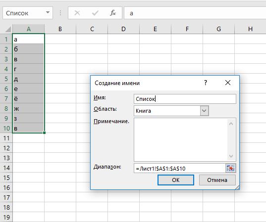
- In the line for entering the name, indicate the name of the future list (it will be further used in the formula for substitution). Please note that it must begin with a letter and not have spaces.
- Now select one or more cells in which the drop-down list will be created in Excel.
- In the upper pane of the Excel window, click the tab named "Data."
- Go to the "Data Verification" item. The window for checking the input values starts.
- On the Options tab, in the data type line, specify List.
- Next comes the item named "Source" (the value string will not be available for changes). Here you must put an equal sign, and after it, without spaces, the name of the list that you indicated earlier. The result should be "= list". This will allow you to enter only the data that is listed in the list itself. To perform the operation, the specified value will be checked, and the offer of available options will be executed, which are the list.
- In the event that the user indicates the missing data, Excel displays an error message indicating that the entered value does not exist. And if you click on the drop-down list button installed in the cell, a list with options that was created earlier will appear.
ActiveX Enabled
Before implementing this method of creating a drop-down list in Excel, you need to activate a tab called "Developer". This is done in this way:
- Launch the “File” submenu on the top panel of the program window.
- Go to the item called "Options." The settings window will open.
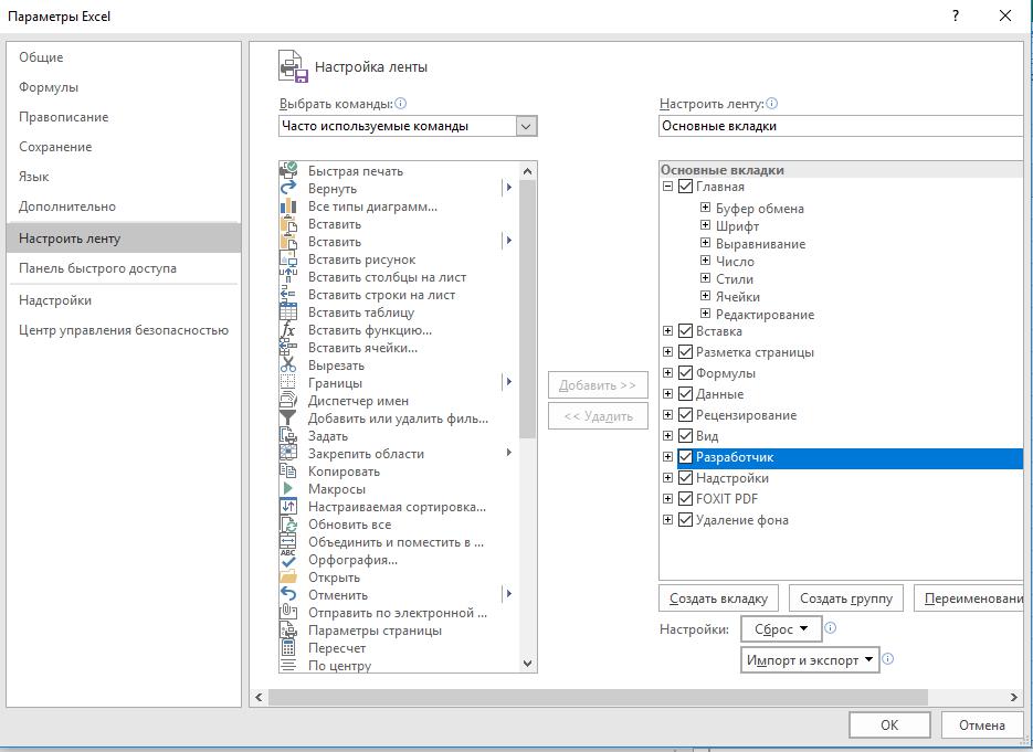
- In its left part there will be a list in which you need to find and run the ribbon settings line.
- Another page will open. In the list on the right, find the "Developer" item and check the box in front of it. After that, it will be possible to use a tool called "Combo Box (ActiveX Element)".
- Now let's move on to the process of implementing the list: open the connected tab "Developer" and select the "Insert" button. A small window with various elements will appear.
- Among them, find the List Box tool specified earlier. It will be located at the bottom of the window, the second in the first row.
- After that, draw this object in the cell where you plan to make a list. Next, it is configured.
- To do this, run constructor mode. It is located in the developer tab. Next, click on the "Properties" button. A special window will start.
- Without closing it, click on the list object created earlier. Next, you will see a lot of different criteria for customization. But you need the following:
- ListFillRange - Defines a range of cells. They will be used to consume list values. Here you can enter several columns at once.
- ListRows - indicates the number of lines to be specified in the drop-down list. Thanks to the launched developer tab, you can specify a large number of positions.
- ColumnCount - adjusts the number of columns displayed by the list.