For economists, it is often necessary to optimize the production function, maximize or minimize it, for example, profit, loss or other data, taking into account the linear constraint. Understanding linear programming problems and setting goals - this requires knowledge of the basics of mathematics and statistics. The task of linear programming (LP) is to define a function to obtain optimal data. This is one of the most important business transaction research tools. It is also widely used as an aid in decision-making in many industries: in the fields of economics, computer science, mathematics, and other modern practical research.
Characteristics of linear programming tasks
The following LP features are distinguished:
- Optimization. The basis of linear programming problems and statement of optimization problems is to maximize or minimize a certain database, which is the subject of research. This is often found in economics, business, advertising, and many other areas that require efficiency in order to conserve resources. This includes issues of profit, resource acquisition, production time and other important economic indicators.
- Linearity. As the name implies, all LP tasks have a sign of linearity. However, it is sometimes misleading, since linearity refers only to variables of degree 1, excluding power functions, square roots, and other nonlinear dependencies. At the same time, it does not mean that the functions of the LP problem have only one variable. It refers to variables as the coordinates of points on a line, excluding any curvature.
- Objective function. The basis of linear programming tasks and setting objective tasks is variables that can be changed at will, for example, time spent on work, produced units of goods. The objective function is capitalized with the letter “Z”.
- Limitations All LPs are limited to variables within the function. These restrictions take the form of inequalities, for example, “b <3”, where b can represent units of books written by the author per month. These inequalities establish how the objective function can be maximized / minimized, since together they determine the areas of decision making.
Conditions task definition
Companies strive to get the highest profitability in their activities, therefore they should make the most of their resources: human, materials, equipment, facilities and others. LP appears to be a useful tool to help determine the best solution in a company.
The conditions for completing linear programming tasks and setting tasks are necessary to obtain maximum net profit. In order to solve the LP problem, it must have:
- Restrictions or limited resources, such as a limited number of employees, a maximum number of customers, or a limitation of production losses.
- Goal: maximize revenue or minimize costs.
- Proportional linearity. The equations that generate the decisive variables must be linear.
- Homogeneity: the characteristics of decision variables and resources are the same. For example, a person’s hours of operation are equally productive or products manufactured on a machine are identical.
- Divisibility: products and resources can be displayed as fractions.
- No negativity: decisions must be positive or equal to zero.
The objectiveness of the function in the formulation of the main linear programming problem mathematically expresses the goal that must be achieved in solving the problem. For example, maximize company profits or minimize production costs.
This is represented by an equation with a variable solution, where: X 1, X 2, X 3, ..., X n are solution variables; C 1, C 2, C 3, ..., C n are constants.
Each constraint is expressed mathematically with any of these attributes:
- Less than or equal to (≤). When there is an upper limit, for example, overtime cannot be more than 2 hours a day.
- Equal (=). Indicates the required relationship, for example, the final stock is equal to the initial stock plus production minus sales.
- Greater than or equal to (≥). For example, when there is a lower limit, the production of a particular product should be higher than the projected demand.
- The general statement of the linear programming problem begins with the setting of constraints.
- Any LP task must have one or more restrictions.
- The positivity of decision variables should be considered within the scope of constraints.
Stages of setting objectives
The general formulation of the linear programming problem and its formulation relates to the translation of a real problem to the form of mathematical equations that can be solved.
The steps of the statement of the integer linear programming problem:
- Determine the number revealing the behavior of the objective function for optimization.
- Find a set of constraints and express them in the form of linear equations or inequalities. This will establish a region in the n-dimensional space of optimized functions.
- It is necessary to impose the condition of non-negativity on the variables of the problem, that is, all of them must be positive.
- Express a function in the form of a linear equation.
- The function is optimized graphically or mathematically when the mathematical formulation of the linear programming problem is performed.
Graphical way
The graphical method is used to perform LP tasks in two variables. This method is not used to solve problems that have three or more variable solutions.
The standard task is to maximize unknown LP problems, in which the function is increased, subject to restrictions of the form:
x ≥ 0, y ≥ 0, z ≥ 0 and further shape restrictions:
Ax + By + C z +. , ≤ N,
where A, B, C and N are non-negative numbers.
The inequality should be “≤”, not “=” or “≥”.
The graphical LP method with two unknowns is as follows:
- Set possible areas of the graph.
- The angular coordinates of the points are calculated.
- Substitute them in order to see the optimal value. This moment gives a solution to the LP problem.
- The function is minimized and, if its coefficients are non-negative, a solution exists.
Definition of existing solutions:
- Limit the area by adding a vertical line to the right of the rightmost corner point and a horizontal line above the highest corner point.
- The coordinates of the new corner points are calculated.
- Find the corner point with the optimal value.
- If it takes place at the starting point of an unbounded domain, then the LP problem has a solution at this point. If not, then it does not have an optimal solution.
Sketching Solution Set
Select a reference point and mark the area to be blocked.
They draw the area represented by the inequality of two variables in the formulation of the linear programming problem. Briefly for example:
- Draw a line obtained by replacing inequality with equality.
- Select a control point, (0,0). A good choice if the line goes through the beginning.
- If the control point satisfies the inequality, then the set of solutions is the entire area on the same side of the line as the control point. Otherwise, it is on the other side of the line.
- An admissible region is determined by a set of linear inequalities and is a collection of points satisfying all inequalities.
- To draw it, defined by a set of linear inequalities with two variables, perform the areas represented by each inequality on the same graph, not forgetting to shade parts of the plane that are not needed.
Simplex method to maximize
The formulation of the linear programming problem with a mathematical model for maximization can be performed using the simplex method:
- Transform the data into a system of equations, introducing weak variables to turn constraints into equations, and rewrite the function in standard form.
- The source table is recorded.
- Select the heading column, a negative number with the largest value in the bottom row, excluding the far right entry. Its column is a summary. If there are two candidates, choose one. If all numbers in the bottom row are zero or positive, excluding the rightmost record, then everything is ready and the basic solution maximizes the objective function.
- Select the bar in the column. The axis must always be a positive number. For each positive record “b” in the summary column, the ratio “a / b” is calculated, where “a” is the answer in this row. From the test coefficients choose the minimum, then the corresponding number "b" will be the axis.
- Use the bar to clear the column in the usual way, making sure that you follow the instructions for formulating the row operations described in the Gauss-Jordan manual, and then swap the column with the label from the column.
- The variable that originally denotes the summary row is outgoing, and the variable denoting the column is inbound.
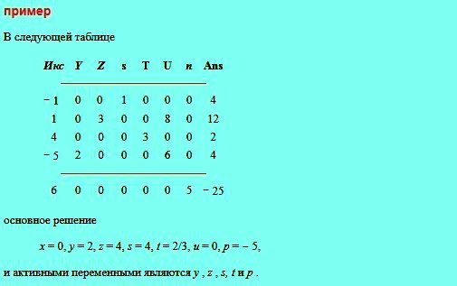
In order to get a basic solution that matches any table in the simplex method, all variables that are not displayed as line labels are set to zero. The value of the displayed row label (active variable) is the number in the rightmost column of the row divided by the number in this row in the column labeled with the same variable.
Custom restrictions
In order to solve the LP problem with constraints of the form (Ax + By +., .≥ N) with positive N, the extra variable is subtracted from the left side (instead of adding a weak variable). The basic solution corresponding to the source table will not be feasible, as some of the active variables will be negative. Therefore, the rules of the initial turn are different from the above.
Next, mark all lines that give a negative value for the associated active variable, except for the target. If there are marked lines, you need to start from stage I.
I stage. The first line finds the largest positive number. Use test factors, as in the previous section, to find a summary in this column, and then expand this entry. Repeat until the marked lines remain, then proceed to step II.
Stage II uses the simplex method for the standard maximization problem. If there are any negative values in the lower left row after stage I, use the method of standard maximization problems.
An example of a game that can be solved using the simplex method.
PHPSimplex Online Tool
Currently, technological tools facilitate many types of professional life activities and LP problem solving methods are no exception. Their advantage is that you can get the best solution from any computer with Internet access.
PHPSimplex is an excellent online tool for solving LP problems. This application can solve problems without restrictions on the number of variables and restrictions. For tasks with two variables, he demonstrates a graphical solution and presents the entire process of calculating the optimal solution in a simple and understandable way. It has a user-friendly interface, is close to the user, easy to use and intuitive, available in several languages.
WanerMath: Applications Without Borders
Warneth provides 2 tools for solving linear programming problems:
- Linear programming graph (two variables).
- Simplex method.
Unlike other tools where only coefficients are placed, all functions with variables are included here. This does not present much difficulty for novice users, as there is a user manual on the profile site. In addition, the site has the “Examples” function, which automatically creates tasks so that the user can evaluate his work, for example, when setting the transport linear programming problem.
JSimplex is another online tool. It allows you to solve LP problems without limiting the number of variables. It has a simple control interface, in which it is proposed to indicate the purpose and number of variables. The user records the coefficients of the objective function, the constraints and clicks on “solve”. It will show the integration, calculation of the best option and the results of each variable.
As you can see, these tools are extremely useful for easily learning linear programming solution procedures.
Simple LP Example
The company produces portable and calculators for scientific work. Long-term forecasts indicate the expected daily need for 150 scientific and 100 portable calculators. Daily production capacity daily allows you to produce no more than 250 scientific and 200 portable calculators.
In order to fulfill a delivery contract, a minimum of 250 calculators must be issued. The implementation of one - leads to a loss of 20 rubles, but each handheld calculator makes a profit of 50 rubles. It is necessary to perform the calculation in order to get the maximum net profit.
The algorithm for executing an example of setting linear programming problems:
- Variable solutions. Since the optimal number of calculators was specified, they will be the variables I in this task: x - the number of scientific calculators, y - the number of portable.
- Set limits, because the company can not produce a negative number of calculators per day, the natural limit will be: x ≥ 0, y ≥ 0.
- Lower bound: x ≥ 150, y ≥ 100.
- Set an upper bound for these variables due to company production restrictions: x ≤ 250, y ≤ 200.
- Joint restriction on the values of 'x' and 'y' due to the minimum order for shipment: x + y ≥ 250
- Optimize the net profit function: P = -20x + 50y.
- Solution: maximize P = -20x + 50y, provided that 150 ≤ x ≤ 250; 100 ≤ y ≤ 200; x + y ≥ 250.
Areas of use
Among the applications of linear programming, the most common are:
- Aggregate sales and operations planning. The goal is to minimize production costs in the short term, for example, three and six months, satisfying the expected demand.
- Product planning: find the optimal combination of products, given that they require different resources and have different costs. As an example, you can find the optimal mixture of chemical elements for gasoline, paints, diets for humans and animal feed.
- Production flow: determine the optimal flow for the production of the product, which must pass sequentially through several work processes, where each has its own costs and production characteristics.
- Statement of the linear programming transport problem, transportation schedule. The method is used to program several routes of a certain number of vehicles to serve customers or to receive materials that will be transported between different places. Each vehicle can have a different payload and performance.
- Inventory management: determining the optimal combination of products that will be available in stock in the sales network.
- Personnel programming: development of a personnel plan that can satisfy the expected variable demand for specialists with the minimum possible number of employees.
- Waste control: Using linear programming, you can calculate how to reduce waste to a minimum.
These are some of the most common applications where linear programming is used. In general, any optimization problem that satisfies the above conditions can be solved with its help.