When preparing reporting documentation, sometimes it is necessary to use the summation of cells that meet certain conditions. So, the function "sumslimn" in Excel (examples will be given) does an excellent job of the task. If the “summed” operator allows selection according to one condition, then the above option allows you to use several ranges.
Math functions in Excel
This category contains about 80 functions. Here you can find operators that can calculate the values of a spreadsheet of any format. In Excel, sums are common, and a set of trigonometric functions is suitable for a certain circle of users. What is expressed the essence of the arithmetic operator, which has an analogue in the latest versions of the software "sumslimn"? Its task is to summarize the values that fall under certain criteria.
To a greater extent, mathematical functions are designed to automate the user's work. If you have questions about the use of the operator, call for help. You can do this in the “Function Arguments” window by clicking on the “Quick Reference” link or through F1.
To enter the formula, you must first click the "=" sign. Otherwise, the software recognizes the information as text or generates an error. The user prescribes formulas manually, relying on his knowledge and skills, through the toolbar or through the "Substitution Wizard".
Function Description
The sum of numbers that satisfy certain criteria is achieved through the "sumlims" operator in Excel. Examples, if you consider, clearly show how to properly use this function and avoid mistakes.
In the VBA programming language and the English version of the spreadsheet editor, syntax written in Latin letters is adopted. In the domestic counterpart - Russian.
The syntax of the function is as follows: = sum sum (sum_range; [condition_range1; condition1]; [condition_range2; condition2]; ...)
The summation range is understood as an array whose cells will be added if they satisfy the following conditions. Another block of arguments in the syntax is condition_range1; condition 1. They allow you to select the necessary cells in a specific array by the first factor, which are subsequently summed up within the original interval. Additional criteria are the following condition_range10; condition 10.
Feature Features
- If we compare the "sums" and "sums", then the location of the arguments in the syntax of the specified operators is different. The first function has the summation range in the third position, the second - in the first.
- If you incorrectly enter the data for the "sumlim" in Excel, the examples detect an error. The fact is that the dimension of all rows and columns of ranges is the same for this operator. Summesli allows a different number of cells in the summation interval and conditions.
- In the case of enumerating the first argument, empty or text cells are detected, they are ignored.
- When prescribing the criterion, the sign “*” is used. It means that you need to search for the contained fragment and not one hundred percent match with the condition.
- The function "sumslim" in Excel (examples confirm this) allow string lengths up to 255 characters.
- The cells indicated in the summation range only add up when they satisfy all the conditions set. In other words, the logical function “AND” is also performed.
Example 1
To consolidate the material, the user needs to solve such problems by “total limit” in Excel. Examples of use are presented below.
5 columns are given where:
- date;
- color;
- state;
- quantity;
- cost.
Searches by the following criteria:
- summation range: F5: F11;
- interval of the first condition: search by color;
- initial selection criterion: contains the word red;
- range of the second condition: state search;
- another criterion: abbreviation TX is contained.
Example 2
4 columns are given in which are indicated:
- A - product category;
- B - specific products;
- C is a Russian city;
- D - sales volume.
The first condition in example 1 is to select all cells containing the word “vegetables”. The second criterion is to find the cells responsible for the city of Moscow. In the second example, the first condition contains a fruit search. The second criterion relates to Kazan.
In order to correctly write the “summax” formula in Excel, examples recommend that the conditions be put in separate cells. Thanks to this, the user refers to a specific address, which eliminates an error in the function.
In the second statement, the digits indicate the sum sumlim argument:
- 1 - summation range (sales volume);
- 2 - interval of the first condition (search by category);
- 3 - criterion 1 (search for the word "fruit");
- 4 - range of the second condition (finding in the city);
- 5 - criterion 2 (search for the word "Kazan").
Example 3
2 columns are given. The first shows the names of employees, the second shows the sales for each of them. It is necessary to create 3 functions "sumslimn" in Excel. Examples of how to do this are shown in the image.
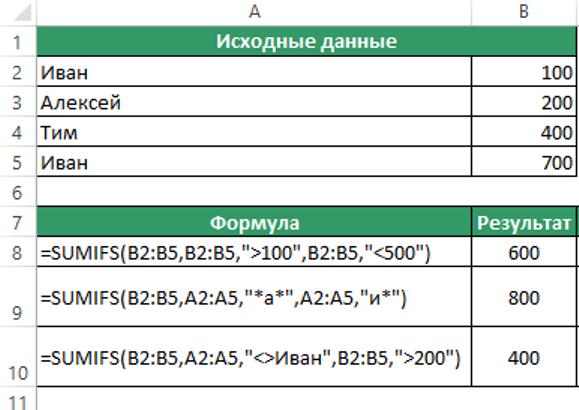
- The summation range is indicated for the first operator (it is the same for all three functions): B2: B5; the interval of the first and second conditions coincides with the previous one, the first criterion selects the rows where the sales volume is not less than 100, and the second - where not more than 500.
- For the second operator, the previous summation range is indicated. The first column is a selection of conditions: the first talks about finding names that contain the letter "a", the second - finding a seller whose name begins with "AND". The found values are summarized.
- For the third operator, the previous summation range is also indicated. For both conditions, the search is in the first column. Initial selection criteria: seller’s name "<> Ivan". The second condition: sales of more than 200.
Example 4
Given 3 columns, which indicate the date, type of expenses, the amount for a specific type of spending. It is necessary to make a selection according to two conditions:
- The criterion does not include the word “Other”.
- The condition contains the word "Expenses *". The sign “*” indicates that after the entered information there is a continuation in the cell of column B.
As an independent task, the user can enter a condition by the date for a specific period: for a month or a week. To do this, you must specify the period in quotation marks, for example, "> 01/01/2017". The second condition is: "<01/31/2017."
Excel features are always detailed in Microsoft Help. If questions arise, even an experienced user does not hesitate to apply the built-in help of the program.